

In this post, we build a simple stock market simulation to use for retirement planning.
I am a long way from retirement, but how much is enough for retirement? There are certainly lots of financial advisors who will let you pay them to tell you the answer. There are also rules of thumb, including:
- The 4% rule: In your first year of retirement, add up all your assets and withdraw 4%. In subsequent years, adjust this number for inflation.
- Save 10-15% of income until retirement.
- Aim to save 25x of your annual spending by retirement.
- Hold (100-your age)% in stock.
However, are these enough, and what happens if we have a long-lasting, high inflation environment? In addition, I don’t really want to get to retirement only to find my assumptions were incorrect. Therefore, I wanted to create a simulation that we can use to create and test different retirement models. Then we can run the simulation in expected and extreme cases (recession, stock market crash, inflation), to see how resilient each model would be.
Our starting point will be to model the stock market. As a very important note, our stock market model will only look at annual returns over a long period of time. It should not be used for actual investing. Our notebook code is available in our Github repository.
The Data
We will start by collecting annual stock market data (or you could just use the collected data in our repository). We will use the S&P 500 for a few reasons. The S&P 500 includes the 500 largest companies across many different sectors. The cross-sector nature helps to reduce volatility for a specific sector (although information technology is increasingly a larger percentage of the index).
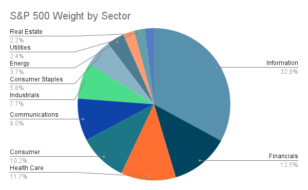
Second, the S&P 500 has many, easily available exchange traded funds (ETF), and Warren Buffet famously showed that an index ETF is an effective investment strategy.
Kaggle has historical S&P 500 data (1927 to 2020). This data is more granular than we need; therefore, I converted the data from daily into annual data, selecting the first trading day of every year. I added a column for year over year percent change and a column for log change (I am experimenting with this column).
Next, using Pandas, we load the data and plot it.
import pandas as pd
import numpy as np
import matplotlib.pyplot as plt
import seaborn as sns
import scipy
spx = pd.read_csv("https://raw.githubusercontent.com/harlepengren/DataAnalysis/main/data/SPX_annual.csv")
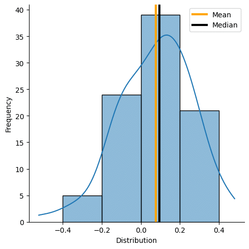
ax = sns.displot(spx["Change"],bins=[-0.4,-0.2,0,0.2,0.4],kde=True)
ax.set(xlabel='Distribution', ylabel='Frequency')From the histogram, we see that it is a left skewed distribution. The term left skew is confusing since the line appears to lean toward the right. In this case, left refers to the fact that the mean is to the left of the median due to a long left tail.
[histogram with mean and median plotted]
The Model
Now that we can model the stock market. Let’s create the simulation model. We will create three classes:
- Stock: This models basic operations of a stock: buy, sell, pay dividend.
- Model: A generic model that we can use for different classes of assets (e.g., bonds).
- StockModel: Handles the actual simulation.
Stock Class
Starting with the stock class. We will create the following methods:
- Initialization
- Buy (amount): Buy shares equivalent to a currency amount.
- Buy (shares): Buy a specific number of shares.
- Sell (amount): Sell shares equivalent to a currency amount.
- Sell (shares): Sell a specific number of shares.
- Pay dividend: Pay the annual dividend.
- str: Output a string with stock information.
Here is the full code:
class Stock:
  def __init__(self, ticker:str, price:float, num_shares:float, dividend:float):
    """Initialize the stock:
    ticker: stock ticker (e.g., voo)
    price: price per share
    num_shares: number of shares (note this is float to allow fractional shares)
    dividend: *annual* dividend"""
    self.ticker = ticker
    self.price = price
    self.num_shares = num_shares
    self.dividend = dividend
    self.cost_basis = price

  def pay_dividend(self)->float:
    return self.dividend * self.num_shares

  def buy_amount(self, amount:float):
    """Used if you have a specific currency amount of stock you
    want to buy."""
    self.num_shares += amount/self.price

  def buy_shares(self, num_shares:float):
    self.num_shares += num_shares

  def sell_shares(self, num_shares:float)->float:
    max_shares = min(num_shares,self.num_shares)
    self.num_shares -= max_shares
    return max_shares * self.price

  def sell_amount(self, amount:float)->float:
    """Used if you have a specific currency amount of stock you
    want to sell."""
    sell_shares = amount/self.price
    total_shares = min(self.num_shares,sell_shares)
    income = total_shares * self.price
    self.num_shares -= total_shares

    return income

  def change_dividend(self, percent:float):
    """Change the dividend by a given percentage."""
    self.dividend *= (1 + percent)

  def change_price(self, percent:float):
    """Change the price by a given percentage."""
    self.price *= (1+percent)
    self.change = percent

  def __str__(self):
    return "Price: " + str(self.price) + "\nShares: " + str(self.num_shares) + "\nDividend: " + str(self.dividend) + "\nTotal: " + str(self.price * self.num_shares)
Model Class
Next, we will create the generic model. This only has two methods:
- Initialization: create an empty list for holdings.
- Add: add a holding.
class Model:
  """Basic parent model class."""
  def __init__(self):
    self.holdings = []

  def add(self, new_holding):
    self.holdings.append(new_holding)

  def run_model(self):
    raise NotImplementedError
Stock Model Class
Finally, we create the stock model with the following methods:
- Initialization
- Get Net Worth: Calculate the value of all holdings.
- Get Dividend: Get the stock dividend for all the holdings.
- Get Stock Change: Allows access to how much the stocks changed year over year.
- Run Model: self explanatory.
- Basic Test: Runs the model with 1 stock for a certain number of years.
class StockModel(Model):
  def __init__(self):
    self.spx = pd.read_csv("https://raw.githubusercontent.com/harlepengren/DataAnalysis/main/data/SPX_annual.csv")
    self.dividend = pd.read_csv("https://raw.githubusercontent.com/harlepengren/DataAnalysis/main/data/SPX%20Yield.csv")
    self.dividend["Yield"] = self.dividend["Yield"].str.rstrip('%').astype('float')/100.0
    self.stock_stats = scipy.stats.skewnorm.fit(self.spx["Change"])
    self.dividend_stats = scipy.stats.skewnorm.fit(self.dividend["Yield"])

    super().__init__()

  # Test whether this is generating accurate stock numbers
  def basic_test(self,stock_price:float,num_shares:float,years:int)->float:
    """Test whether the model is generating accurate stock numbers."""
    price_list = []
    stock = Stock("test",stock_price,num_shares,0)
    self.add(stock)
    for index in range(years):
      self.run_model()
      price_list.append(self.get_net_worth())

    return price_list

  def get_net_worth(self)->float:
    value = 0

    for current_stock in self.holdings:
      value += current_stock.num_shares * current_stock.price

    return value

  def get_dividend(self)->float:
    total_dividend = 0

    for current_stock in self.holdings:
      total_dividend += current_stock.dividend

    return total_dividend

  def get_stock_change(self)->float:
    return self.stock_change

  def get_dividend_change(self)->float:
    return self.dividend_change

  def run_model(self)->float:
    # Update the stock value
    self.stock_change = scipy.stats.skewnorm(self.stock_stats[0],self.stock_stats[1],self.stock_stats[2]).rvs()
    self.dividend_change = scipy.stats.skewnorm(self.dividend_stats[0],self.dividend_stats[1],self.dividend_stats[2]).rvs()

    income = 0
    for current_stock in self.holdings:
        current_stock.change_price(self.stock_change)
        current_stock.change_dividend(self.dividend_change)
        income += current_stock.pay_dividend()

    return round(income,2)
To run the basic test, we will select a random row from our stock data and use that as the starting price. We then run the model with that start price.
Comparison_period = 20
comparison_date = spx[:-comparison_period].sample()
starting_price = comparison_date["Close"].values[0]
index = comparison_date.index.values[0]

comparison = spx.iloc[index:index+comparison_period]

stocks = StockModel()
result = stocks.basic_test(starting_price,1,comparison_period)[-1:][0]
We can compare the result to the comparison. However, for one test it is not likely to be close. Instead, we need to simulate it many times. In my case, I ran this test 100 times. This gives us exactly what we want. An individual test is fairly random, but long term the results approximate the stock market.
Other Assets
We create similar models for bonds and real estate. We won’t go into detail here, but we used data from the US Federal Reserve (bonds and real estate).
Conclusion
Now that we have a mode to simulate assets, we want to run the model with different strategies to see which is the most effective and ensures the assets will last for all of retirement. In a future post, we will talk about building the different models and testing.