Recently, Blender added a simulation node to the geometry nodes. This adds exciting capabilities to geometry nodes. However, this meant that I needed to learn geometry nodes. Prior to this, I knew almost nothing about geometry nodes. I thought the best approach to start was to let my creativity run. Therefore, I created a few test animations.
In this post, I will provide a quick overview of each animation. If there is a particular animation that you are interested in learning more about, leave a comment below.
Atom Model
The first idea was to create a model of an atom (Bohr model).
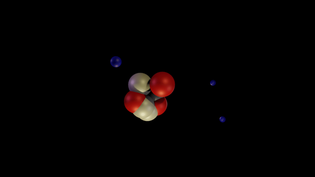
There are two parts to the geometry nodes:
- Neutrons and protons (the center of the model)
- Electrons
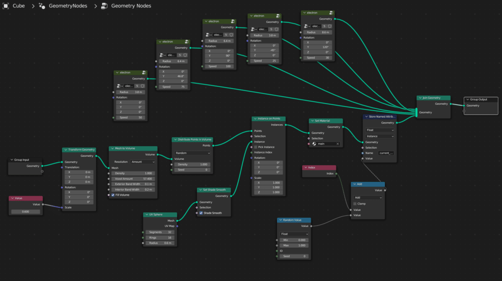
Here are the full geometry nodes:
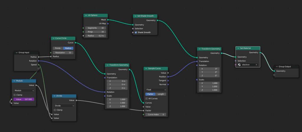
And the electron group repeated for each electron:
Neutrons and Protons
To create the neutrons and protons, we start with the default cube. We convert the cube to a volume and distribute points in the volume.
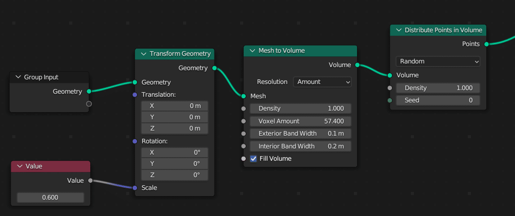
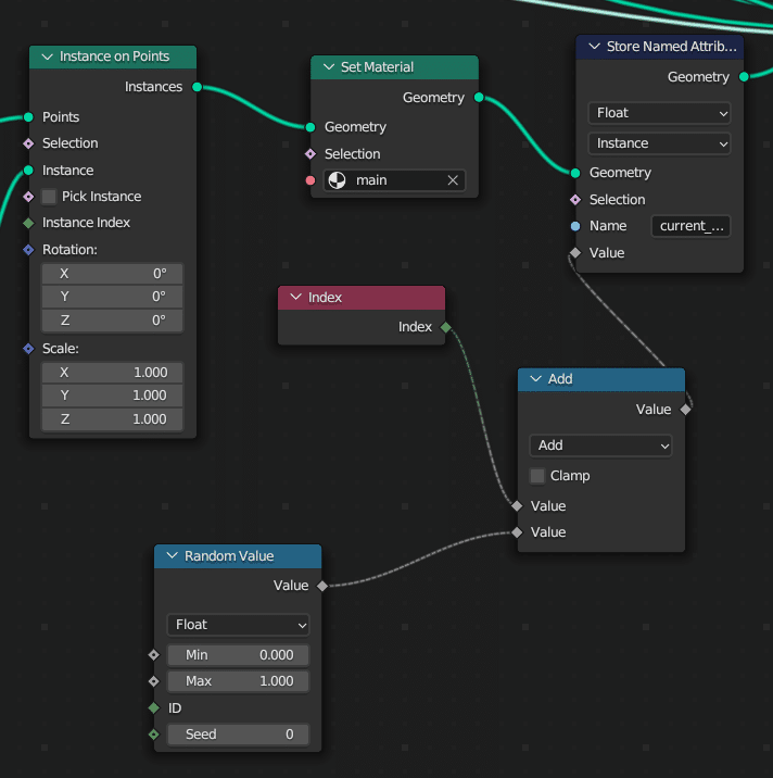
We create a UV sphere on those points and assign the main material.
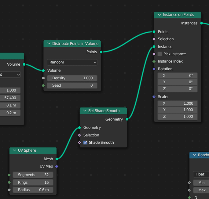
We also assign an index to each one that we use in the Store Named Attribute node to distinguish between the neutron and proton colors (red and white).
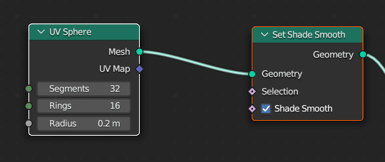
Electrons
For the electrons, we need both the geometry as well as the motion of the electron. To keep the nodes simple, we created a node group for the electrons. We start by creating the sphere.
Next, we create a curve circle and set a starting rotation.
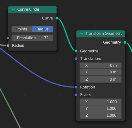
We use the node Sample Curve to get a position along the curve. The position along the curve is determined by the factor input. This input ranges from 0 (beginning of the curve) to 1 (end of curve). We use a speed input to the node group as well as the modulus of the current frame number as the position.
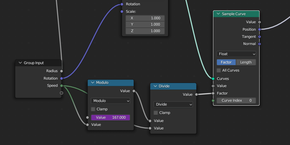
We feed the circle position into a Transform Geometry node and then set the material.
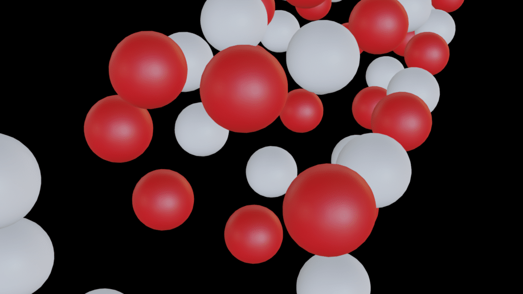
DNA Strand
The second animation is a rotating DNA strand.
Here are the full nodes.
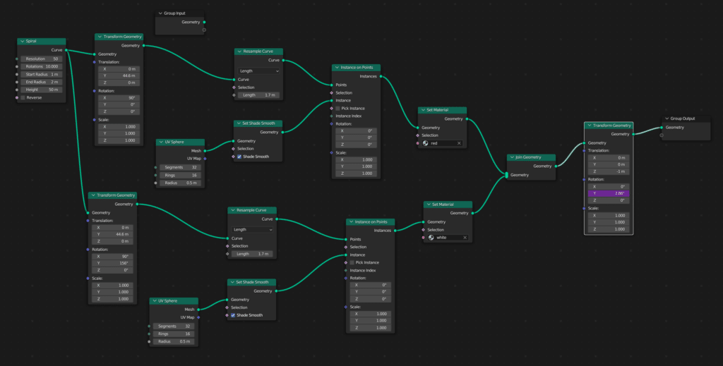
We start by creating a spiral curve and setting the position of the curve.
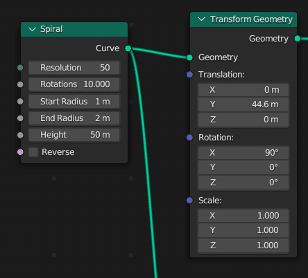
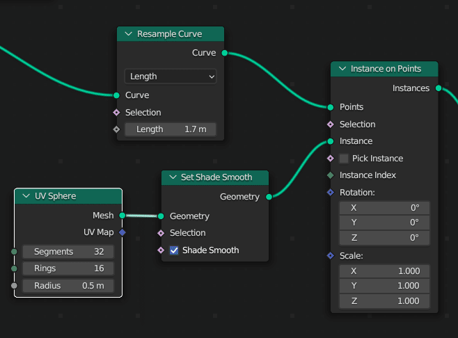
Next, we resample the curve and feed as input into instance on points. This creates points along the curve. You can adjust the number of points based on the length input in the resample node. A smaller length places the points closer together.
We also create a UV sphere and use that as an input to instance in the Instance on Points node.
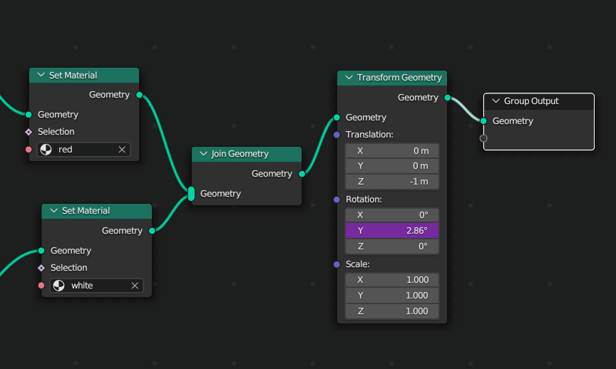
We duplicate most of the nodes to create the second strand. We offset the Y rotation by 156 degrees and give it a different material. We use a join material node to combine the two.
Finally, we add a Transform Geometry node at the end and we animate the Y rotation to create the animation.
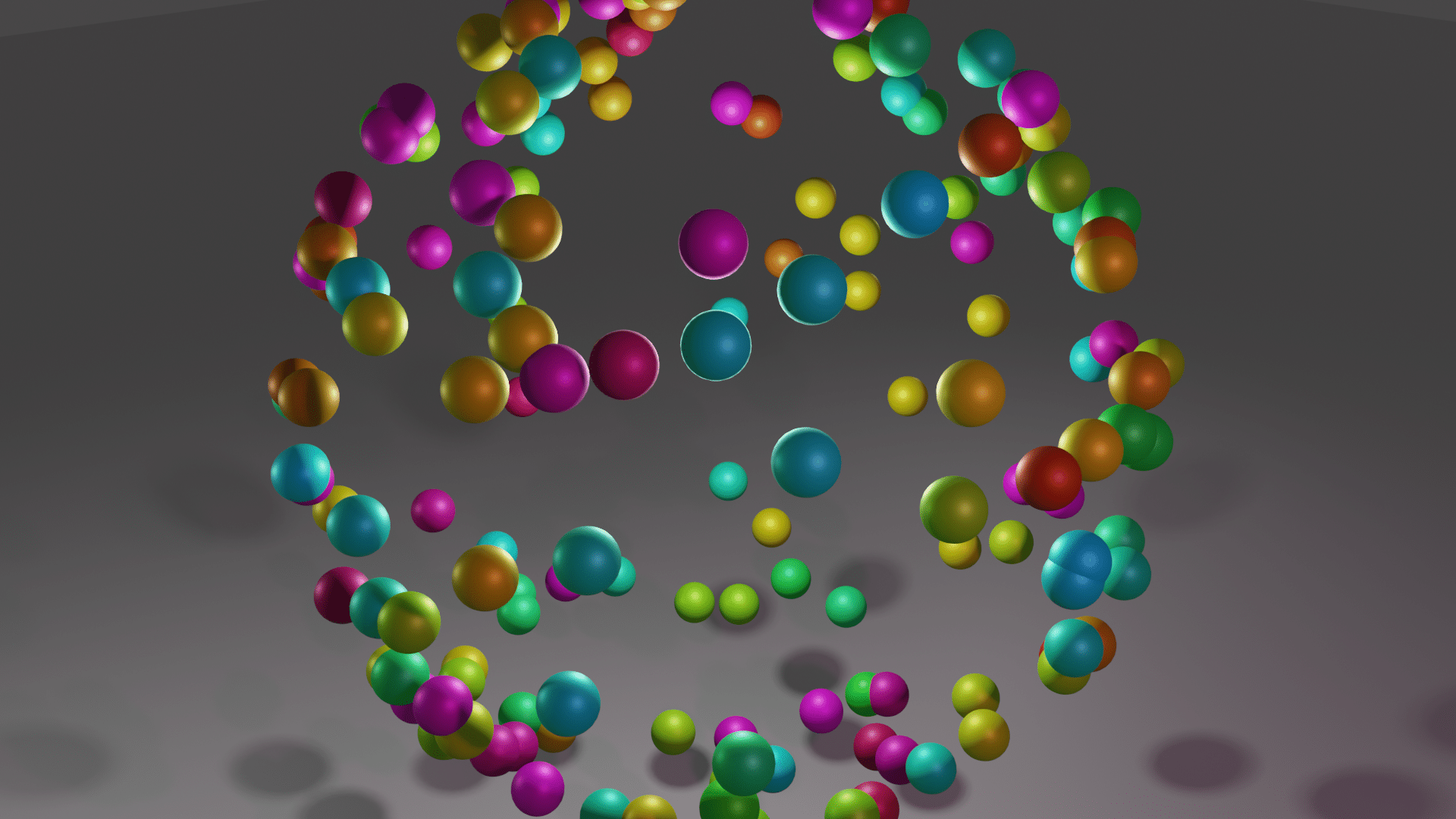
Sphere of Spheres
The next example creates a growing and shrinking sphere composed of smaller spheres.

Here are the full nodes.
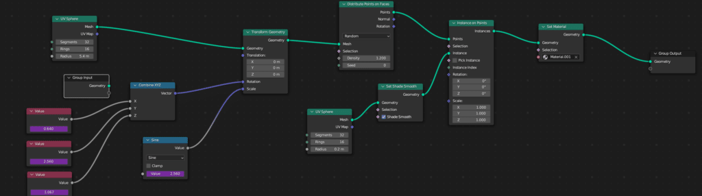
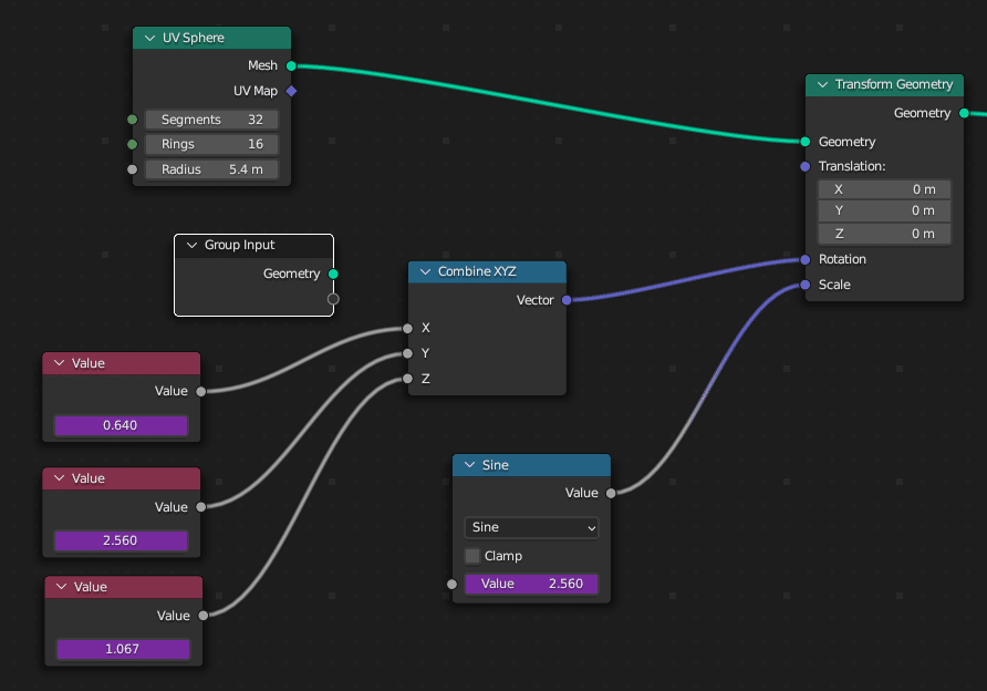
Create a sphere node and a transform geometry node. We will animate the rotation and scale. For the rotation, we simply create three values and feed these into a Combine XYZ node. We animate the three values with drivers. In this case, there is a shortcut to create drivers #frame/100 creates a driver that takes the current frame number and divides by 100. For the scale, we add a math node that we change to sine. The input is another driver, #frame/25.
Next we add a Distribute Points on Faces node that places points at random spots on the sphere. The density setting determines how many points are generated. We input this into Instance on Points node, which we use to convert the points to spheres.
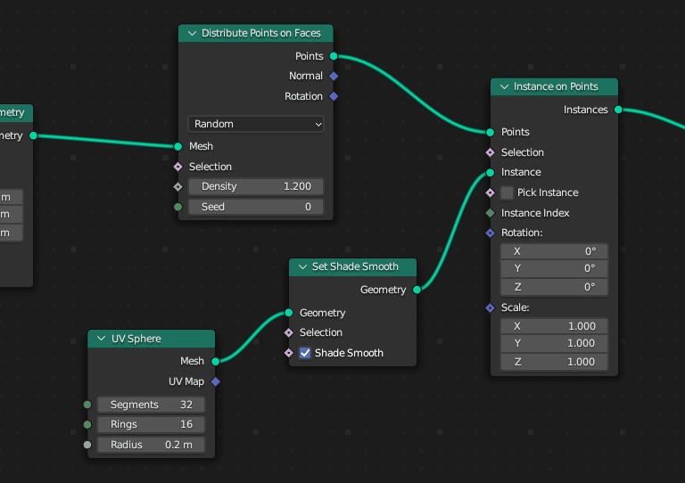
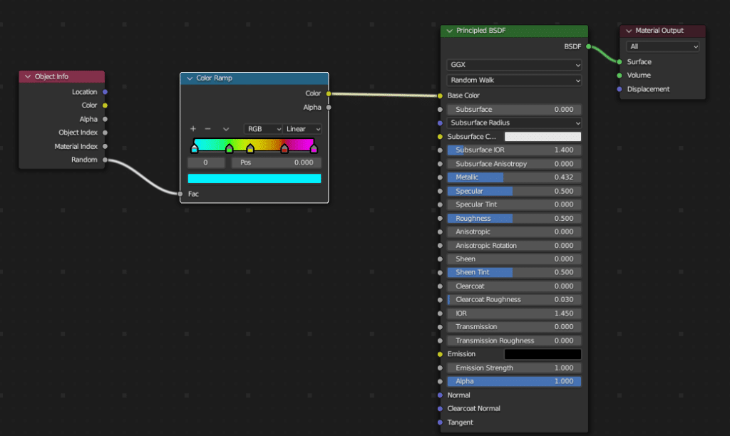
Finally, we set the material through the Set Material node. The different colors of the spheres are set by the material. Here are the shader material nodes.
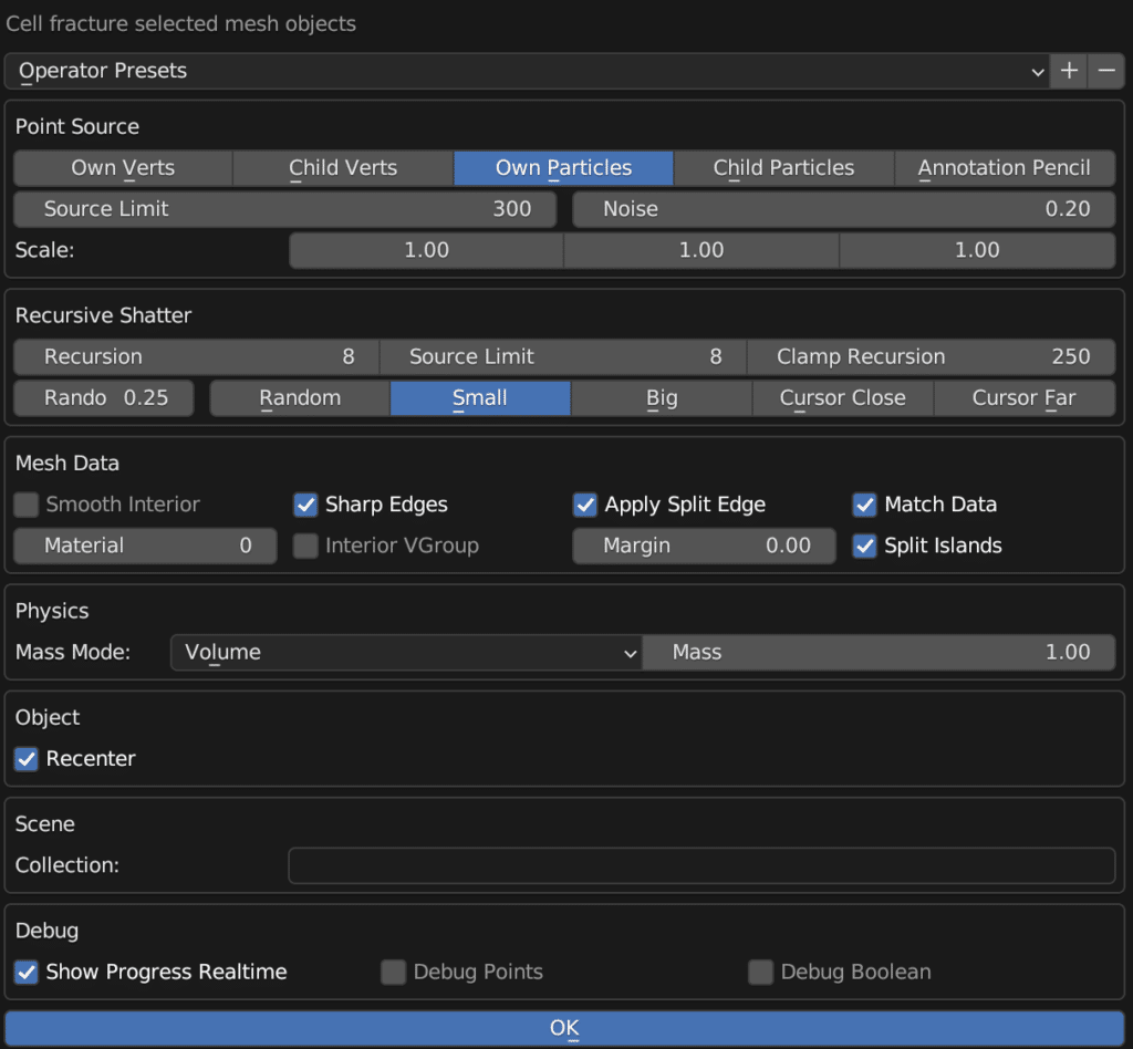
Fracture Assemble
The final example uses the cell fracture addon. Starting with a UV sphere, press the spacebar to bring up the operator search menu. Type “cell fracture” and select the cell fracture operator. I used the settings below.
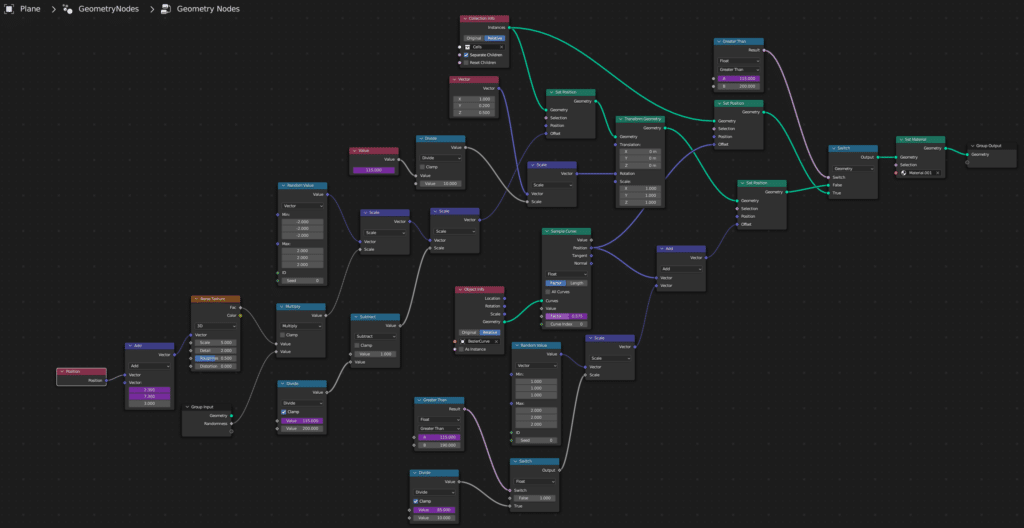
Move all of the fracture objects into their own collection (shortcut m -> new collection). Next, add a bezier curve. We will use this for the path of the fractured elements. Add geometry nodes to the sphere.
Here is the full node setup that we will use.
Move the Object Along a Curve
Add a Collection Info node and select the fracture cell collection that you created. Connect the output of Collection Info into a Set Position node and a Transform Geometry node that we will use later.
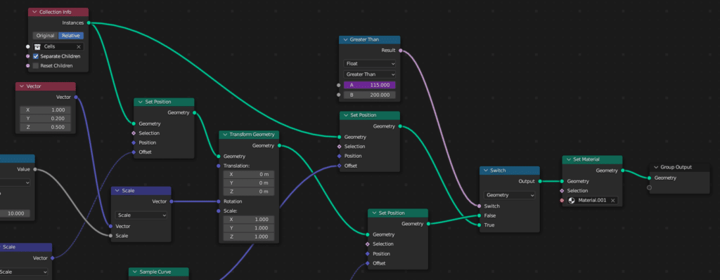
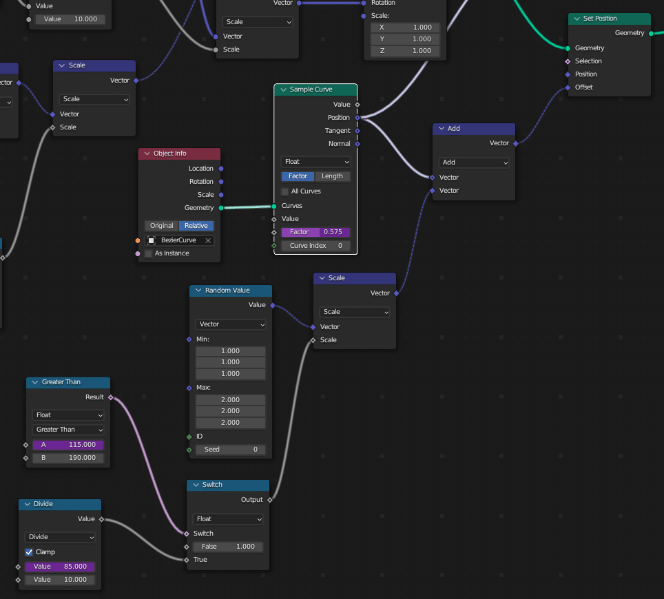
Next, add an Object Info node and set it to the bezier curve. Add a Sample Curve node. In the position input, add a driver “#frame/200”. Take the position output and connect to the last Set Position node offset.
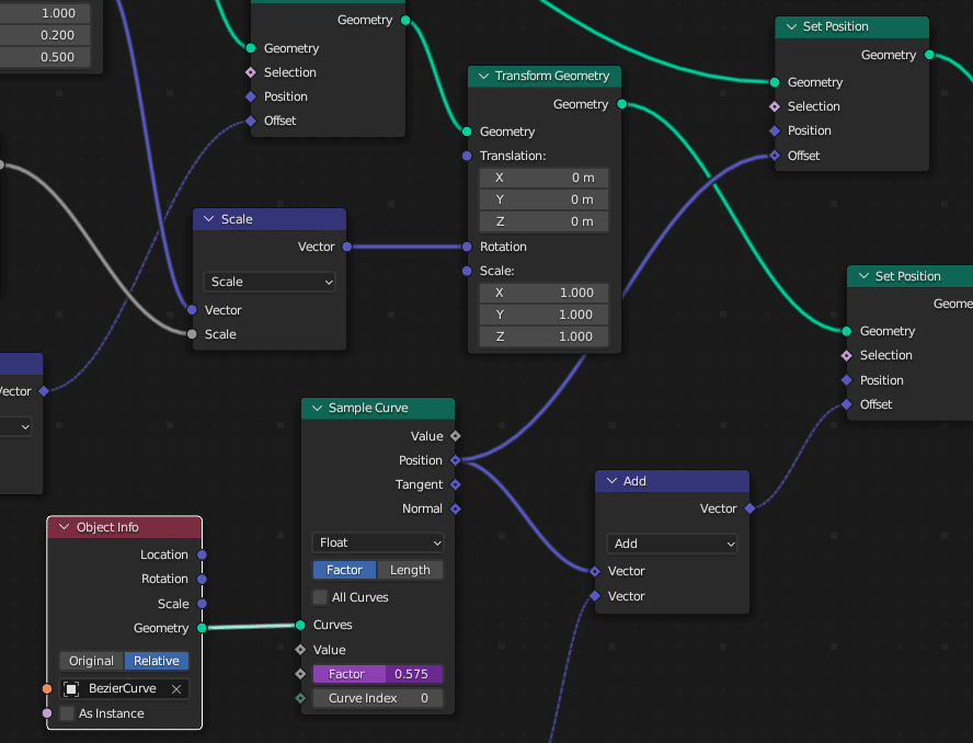
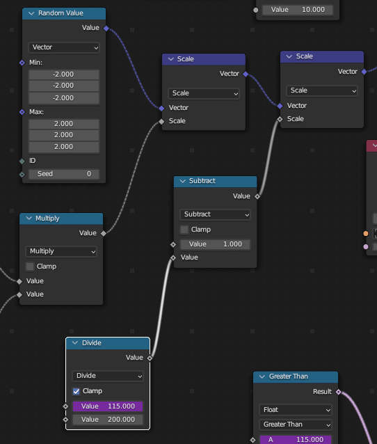
Using a Random Value node, a scale node, and a vector add node, we add a little randomness to the position. We use a switch node to decrease the randomness after frame 200 (as the animation ends).
Final Frames
As we get to the end of the animation, we want the pieces to fly into place. Therefore, we will use a Noise Texture node. We want to animate, so we feed a position node into a vector add. We animate the vector add using “#frame/50” for the X value and “#frame/50+5” for the Y value. The factor output of the texture goes into a multiply node where we multiply it against a float value that we added for the geometry nodes called “Randomness”.
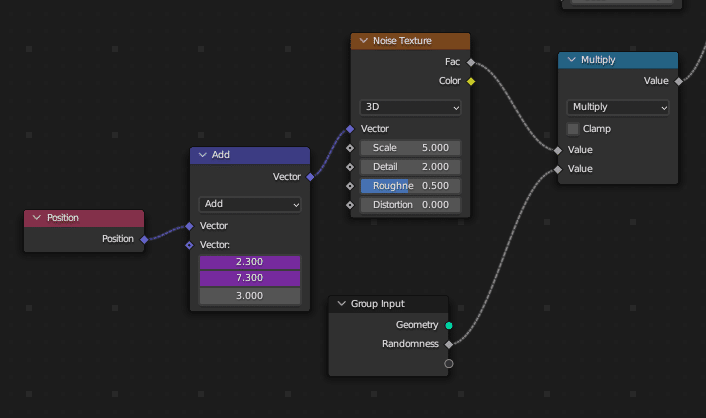
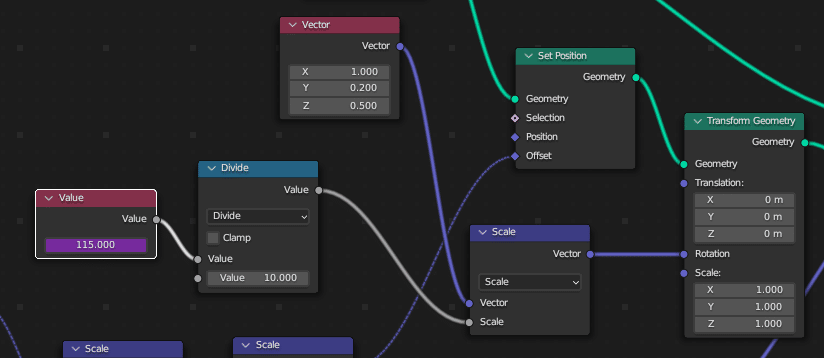
We use the noise to scale against a random value. We then scale again based on how close we are to the end of the animation. We use this as an input into the first Set Position node after the fracture cells Collection Info node.
The last step is to add rotation. We add rotation using the current frame divided by 100. We scale against a starting rotation vector (1, 0.2, 0.5). This is used as an input into the Transform Geometry Node that we added above.
Conclusion
I greatly enjoyed playing with geometry nodes in Blender. Hopefully, you found this useful. We welcome any comments or suggestions in the comments below.