While looking at Pintrest shaders, I found one created by Blender 3D that was mesmerizing. I wanted to recreate it using Open Shading Language (OSL).

The Node Version

Before I created the shader in Open Shading Language, I replicated the node version both to understand how the shader worked and to have a render comparison example. Below is a comparison between the node version and our OSL version. The top is the node version and the bottom is our OSL version.

The Open Shading Language Code

You can download the full code from our Github repository.

Voronoi

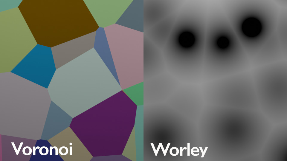
We start with the Voronoi texture. I took a look at the Blender documentation and learned that the Voronoi in Blender is actually a Worley noise texture. I then started down a path to understand the difference. I discovered that Worley noise gives you a cellular pattern whereas in the Voronoi texture, each cell gets its own color. 

Open Shading Language does not include a Voronoi (or Worley) texture in the specification. However, as I looked online for an example Voronoi shader, I discovered that the Blender source code includes many of the Blender nodes implemented in OSL (intern/cycles/kernal/osl/shaders). Therefore, I used a condensed version of that code for the Voronoi function in my shader.

/**********************************************************************
Voronoi texture function.
**********************************************************************/
float voronoi(vector coord,
    float smoothness,
    float exponent,
    float randomness,
    string metric)
{
    vector cellPosition = vector(floor(coord[0]),floor(coord[1]),floor(coord[2]));
    vector localPosition = coord - cellPosition;

    float smoothDistance = 8.0;
    vector smoothColor = vector(0,0,0);
    vector smoothPosition = vector(0,0,0);

    // Look at cells to the left, right, up, down, forward, backward to find closest points
    for (int k = -2; k <= 2; k++) {
        for (int j = -2; j <= 2; j++) {
            for (int i = -2; i <= 2; i++) {
                vector cellOffset = vector(i, j, k);
                point pointPosition = cellOffset +
                                        hashnoise(cellPosition + cellOffset) * randomness;
                float distanceToPoint = voronoi_distance(
                    pointPosition, localPosition, metric, exponent);
                float h = smoothstep(
                    0.0, 1.0, 0.5 + 0.5 * (smoothDistance - distanceToPoint) / smoothness);
                float correctionFactor = smoothness * h * (1.0 - h);
                smoothDistance = mix(smoothDistance, distanceToPoint, h) - correctionFactor;
                correctionFactor /= 1.0 + 3.0 * smoothness;
            }
        }
    }

    return smoothDistance;
}

I won’t go into detail around how the function works. You can find plenty of resources on the Internet that explain Voronoi textures. 

For our purposes, you just need to know that the algorithm creates a pseudorandom set of reference points. For each shading point in our image, we then find the closest reference point and return the distance between the two. There are multiple options for distance, but we are only using actual distance.

The Voronoi function takes 5 inputs. The vector coord is the coordinate we are shading. Smoothness determines how smooth or rough the texture is. We do not use the exponent parameter since we are using actual distance. This particular parameter is only used for the Minkowski distance. Randomness is used to move the reference points around. Finally, metric is the type of distance metric we use. Again, we are only using “actual”.

The Voronoi function returns a value between 0 and 1 (as long as smoothness is > 0).

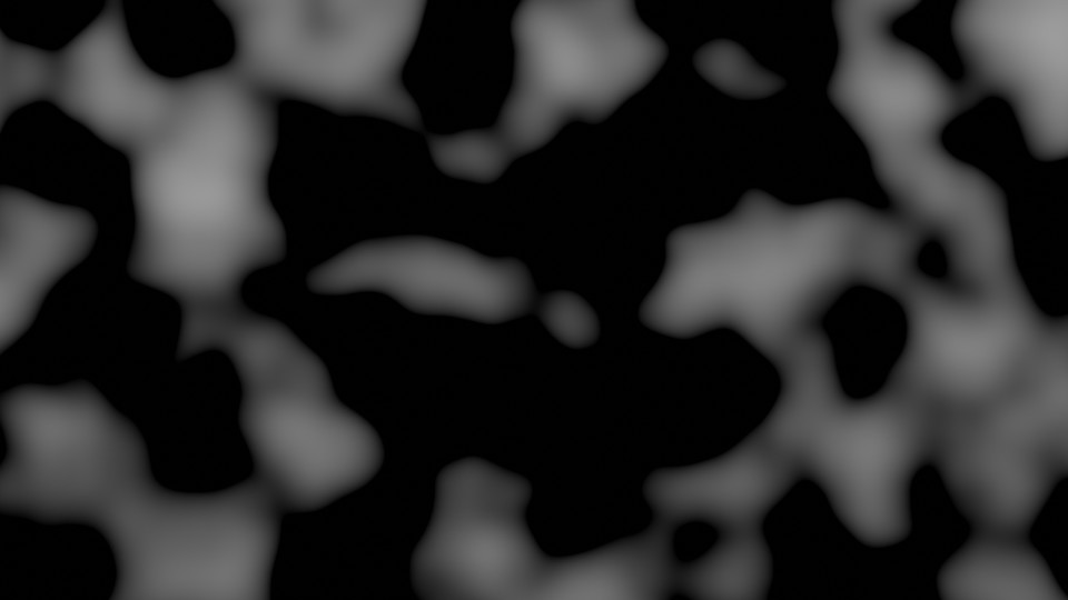
Musgrave

The next texture that we use is the Musgrave texture. According to the Blender documentation, Musgrave is a fractal Perlin texture.

The Blender documentation compares Musgrave to noise texture node by noting that Musgrave texture allows “greater control over how octaves are combined.” The Musgrave texture works by combining multiple different Perlin noise textures together. Each version of the Perlin noise texture is an octave. Lacunarity is the distance between successive octaves.

Again, I started with the Blender source code and simplified it for my purposes.

[code]

float musgrave(point p, float dimension, float lacunarity, float octaves)
{
    float value = 0.0;
    float pwr = 1.0;
    float pwHL = pow(lacunarity, -dimension);

    for (int i = 0; i < int(floor(octaves)); i++) {
        value += noise("perlin",p) * pwr;
        pwr *= pwHL;
        p *= lacunarity;
    }

    float rmd = octaves - floor(octaves);
    if (rmd != 0.0) {
        value += rmd * noise("perlin",p) * pwr;
    }

    return value;
}

The Magic Shader

Now that we have the Voronoi and Musgrave textures, we can create our shader.

The Structure

Our shader will have 10 inputs and 2 outputs. Although, I feel like the longer I spend working on this post, the more inputs I add.

• inputColor: The color of the “magic” inside the glass ball.
• glassColor: The color of the glass ball.
• seed: An input that allows us to change the look of the “magic” inside the ball. 
• vScale: The scale of the voronoi texture.
• vSmooth: The smoothness of the voronoi texture.
• vRandom: The randomness of the voronoi texture.
• mScale: The scale of the musgrave texture.
• threshold: Threshold for the musgrave output.
• density: The density of the absorption within the ball (i.e., it makes inside of the ball darker or lighter).
• IOR: Index of refraction for the glass ball.

The two outputs are:

• surfBSDF: The glass ball surface shader.
• BSDF: The volume shader.

Here is the full code for the shader:

shader magic(
    color inputColor = color(1.0, 1.0, 1.0),
    color glassColor = color(1.0, 1.0, 1.0),
    float seed=1.0,
    float vScale=1.0,
    float vSmooth=1.0,
    float vRandom=1.0,
    float mScale=1.0,
    float threshold=0.55,
    float density=1.0,
    float IOR=1.4,
    output closure color surfBSDF = 0,
    output closure color BSDF = 0)
{
    
    // Volume
    float vor_distance = voronoi((P+seed)*vScale, vSmooth, 1.0, vRandom, "actual");
    float height = ramp(musgrave(vector(vor_distance)*mScale,0.0,1.0,3.0),threshold);

    if(height >= 0.5){
        BSDF = inputColor*height*emission();
    }
    
    BSDF += inputColor*henyey_greenstein(0) + (color(1,1,1)-inputColor)*absorption()*max(density,0.0);
    
    // Glass Outer Shell
    float Kr, Kt;
    vector R, T;
    fresnel(I,N,IOR,Kr,Kt,R,T);
    
    surfBSDF = glassColor*microfacet_ggx(N,0.1)*Kr + glassColor*microfacet_beckmann_refraction(N,0.0,IOR)*Kt;
    
}

Calling All Textures

We start by calling our Voronoi and Musgrave textures.

float vor_distance = voronoi((P+seed)*vScale, vSmooth, 1.0, vRandom, "actual");
float height = ramp(musgrave(vector(vor_distance)*mScale,0.0,1.0,3.0),threshold);

Before we call the Voronoi function, we slightly modify the current shading point (P). We first add our seed to the position. This will change the look of the Voronoi texture (as if we are looking at a different shading point). Next we scale the position point.

With the result of the Voronoi function, we next call the Musgrave function. We turn the result from the Voronoi texture into a vector and scale it. Unlike the Voronoi texture, we do not expose many of the parameters as inputs to the overall shader. Instead, we set the dimension to 0, lacunarity to 1.0, and octaves to 3.

The Ramp

Next, I feed the result into a ramp function. This is similar to the color ramp node in Blender.

float ramp(float value, float threshold)
{
    if(value <= threshold)
    {
        return 0;
    }
    
    return (value - threshold)/(1-threshold);
}

The function takes the value that we are ramping and a threshold. Everything under the threshold is output as 0. From the the threshold point to 1, the function outputs a linear value between 0 and 1.

For example, if value = 0.6, the output is 0.11. If the value is 0.8, the output is 0.55.

Combining the Nodes

Next, we will combine three different closures to create the internal magic.

if(height >= 0.5){
        BSDF = inputColor*height*emission();
    }
    
    BSDF += inputColor*henyey_greenstein(0) + (color(1,1,1)-inputColor)*absorption()*max(density,0.0);

First, we check whether the output of our musgrave texture + ramp is greater than 0.5. If so, we multiply the emission closure by our musgrave output. This sets the brightness of the emission. We also multiply against our input color.

Next we add in scatter and absorption. Scatter causes the incoming light to scatter in all directions. Scatter in Blender is called through henyey_greenstein. For me, this is one of the challenges of using OSL in Blender. The name of the scatter function in Blender is different than the name in the OSL specification. This appears to mainly relate to the closures. If you look in section 7.10 of the OSL specification, it notes that renderers may provide additional closures specific to the renderer as well as allow additional parameters and recommends checking the specific documentation for the renderer, which in our case is https://docs.blender.org/manual/en/latest/render/shader_nodes/osl.html.

Absorption absorbs the incoming light (like water). We multiply the absorption by a density. We also invert the input color. The reason for this is that if the wavelengths of a certain color are absorbed, then the complementary wavelengths are reflected.

The Outer Shell

With the inner “magic” complete, we now move to the outer shell. For the outer shell, we are creating a simple glass ball.

We create four variables: two floats and two vectors. These are used to hold the output of the fresnel.

// Glass Outer Shell
float Kr, Kt;
vector R, T;
fresnel(I,N,IOR,Kr,Kt,R,T);
    
surfBSDF = glassColor*microfacet_ggx(N,0.1)*Kr + glassColor*microfacet_beckmann_refraction(N,0.0,IOR)*Kt;

If you are unfamiliar with C/C++, you may wonder how we can get the result from these four variables. The reason is that all arguments in Open Shading Language are passed by reference (see section 6.4.1 of the OSL specification). Pass by reference simply means you are sending the address of a variable as opposed to a copy of the variable. The fresnel function will store the result at the address that you passed. If you want to learn more about pass by reference, see https://www.geeksforgeeks.org/references-in-c/.

I won’t go into the detail of the fresnel function. If you are interested, there are some great materials available that go into significant depth. For our purposes, it is sufficient to know that Kr is the amount of reflection and Kt is the amount of transmission (refraction). These are controlled by our input IOR, which stands for Index of Refraction. If you want the IOR for common materials, see here.

We will use two closures: mirofacet_ggx and microfacet_beckmann_refraction.

microfacet_ggx is a glossy closure. It takes two parameters, the normal and the roughness. We set the normal to the global variable N, which is the surface shading normal at the current point. We set the roughness to 0.1. We multiply this by Kr or the amount of reflectivity for our index of refraction.

microfacet_beckmann_refraction controls the refraction inside the ball. Again, we pass the normal, N. This function takes two other parameters, roughness and IOR. We set the roughness to 0 and the IOR to the same value we used for the fresnel function. We then multiply by Kt or the amount of transmission.

Conclusion

Based on this, I think we end up with a pretty good result.

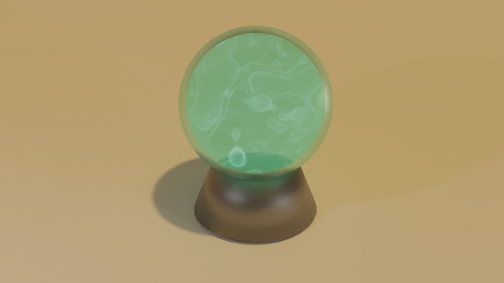
You may ask why it is useful to have an OSL version of something that was much faster to create by nodes. The primary reason is simply continuing our journey to learn shaders generally and Open Shading Language specifically. However, there is also a benefit in terms of control and simplicity. Now that we have the basic shader, we have limitless possibilities that are only confined by our skills in math. For example, We can change the density of the “magic” based on the location within the ball. We may want the center to be very dense, while the outer portion is not dense. In addition, we may want the emission to be very strong in the center but non-existent on the edges. We may be able to do this with nodes, but it would be very complicated and involve many math nodes. Whereas, in OSL, it can be a single line of code.

This leads to the second reason, with our script, we have two nodes: our OSL node and the output node. This compares to the 8 nodes in the node only version. Ours is much cleaner.

However, these benefits come at a cost. OSL only works with CPU Cycles. Therefore, it can be much slower to render.

Hopefully, you enjoyed reading this. I learned a lot in the process of making this. I have several ideas for future posts. If there is another shader that you would be interested in us creating, please leave a comment.