Discover How to Create Scratched Metal OSL Shader in Blender

I found a cool scratched metal OSL shader on GitHub, and I was intrigued for two reasons. First, I am always interested in seeing how different OSL shaders are implemented. Second, it is definitely a useful texture to produce a more realistic texture look.

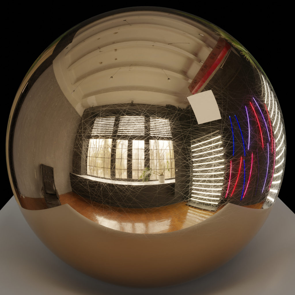
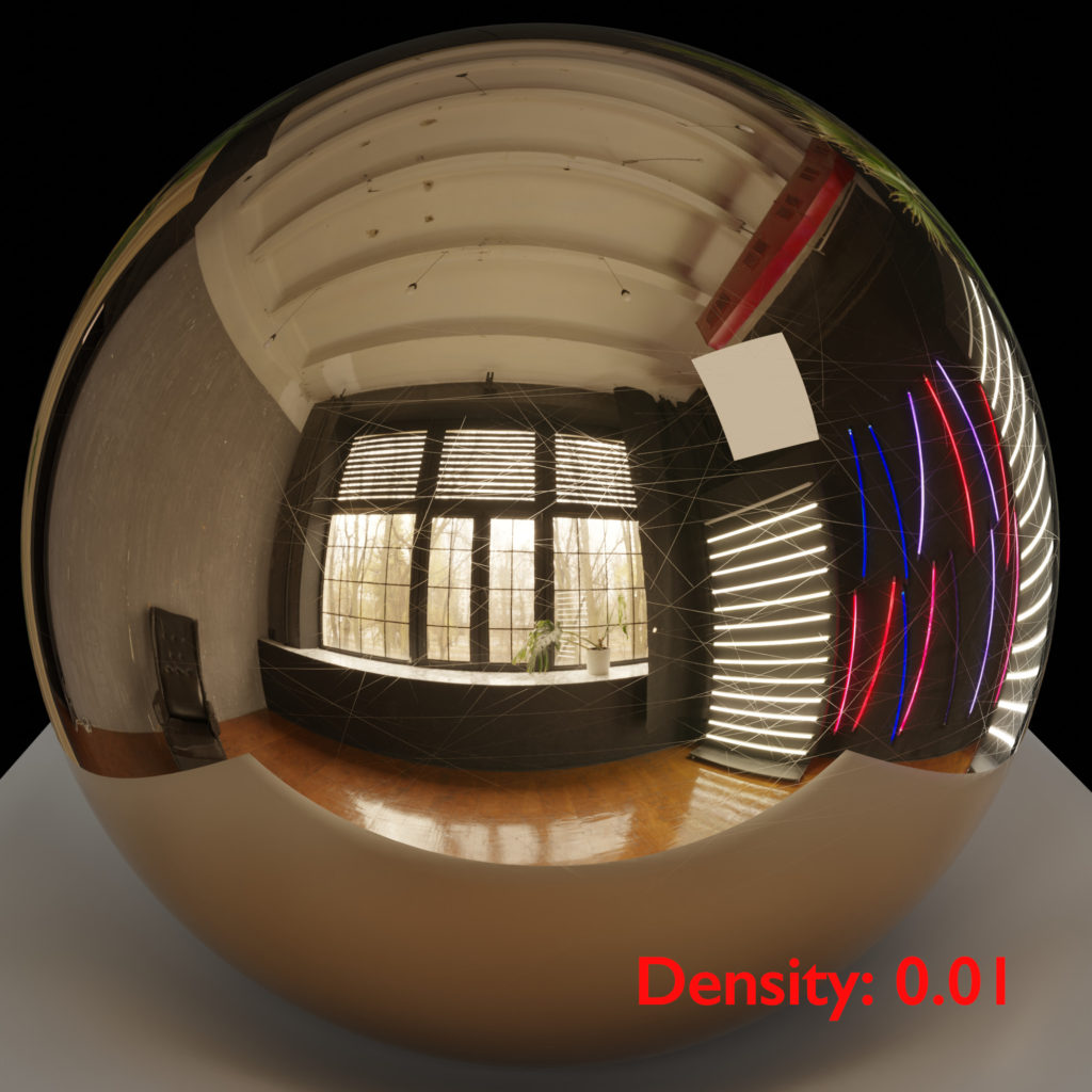
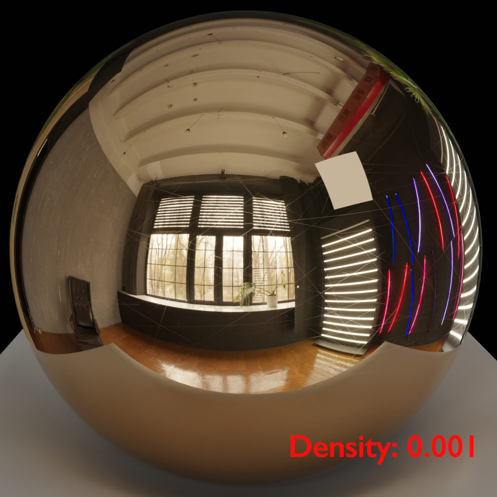
I made some slight modifications to make it work correctly in Blender. Here is an example of the shader. This was rendered with Blender 3.5 using just a basic sphere with the principled BSDF shader and the OSL script that we will discuss below.

In this post, we will talk through how this shader works. For an overview of OSL (Open Shading Language), see our previous post here. For a copy of the Open Shading Language specification, see here.

To understand this shader, we need to understand 4 key components:

• Hashnoise: creating randomness
• Line: the function that makes the scratch
• The Main Body: how we search for a search
• Anisotropy: changing how the scratch affects light

Hashnoise: Creating Randomness

This script makes a few different calls to hashnoise. Hashnoise is a function provided by OSL that creates a type of “random” noise. According to the specification, hashnoise “returns a deterministic, repeatable hash of the 1-, 2-, 3-, or 4-D coordinates.” Deterministic is a fancy way of saying if you use the same inputs you get the same outputs.

For our purposes, the output of hashnoise is random, but in CG, you never want truly random. You want randomness to create the authentic feel, but you want it to be repeatable (deterministic). The image should look the same every time you render the code. Hashnoise gives us this predictable randomness. If we don’t like the look, we can change the input to hashnoise. As soon as we get to an input that creates the look that we like, we know that every time we render we will get the same result.

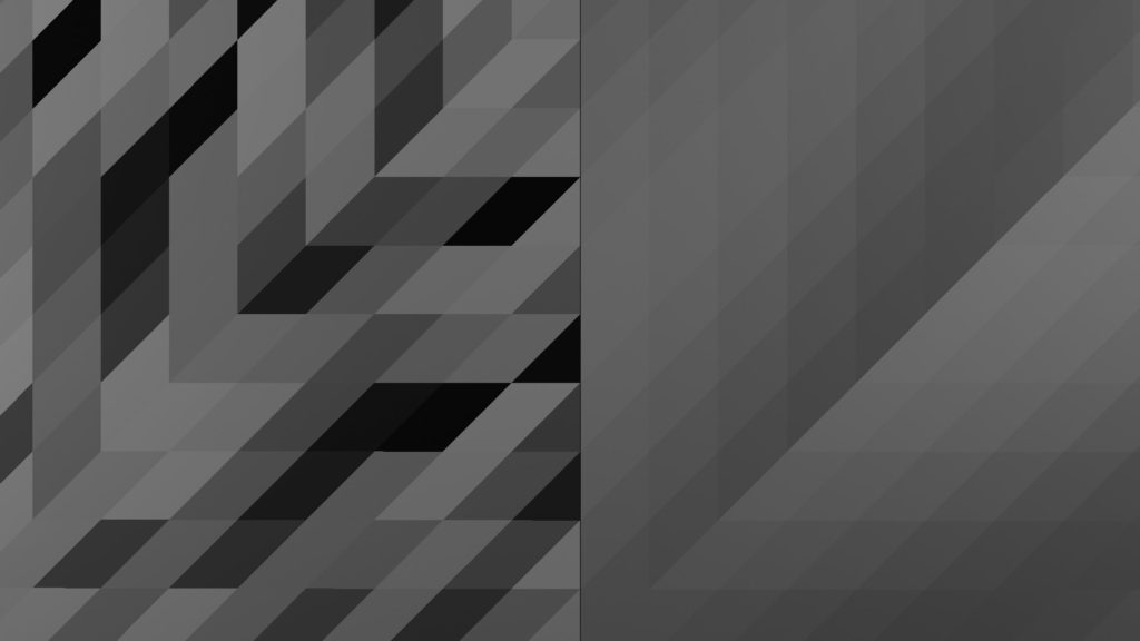
The key difference between hashnoise and perlin noise is that perlin noise is a gradient while hashnoise looks random (the specification says that each point is uncorrelated to the surrounding points). Hashnoise is how old TVs looked when they did not have any signal. To demonstrate, I created two planes and the OSL script below.

shader test(output float hnoise=0.0, output float pnoise = 0.0){
    // Make hnoise big enough to see
    float new_u = floor(u*10.0)/10.0;
    float new_v = floor(v*10.0)/10.0;

    // Create hashnoise and perlin outputs
    hnoise = hashnoise(new_u,new_v);
    pnoise = noise("uperlin",u, v);
}

I assigned the hashnoise output (noise) to the left plane and perlin noise (noise) to the right with the following result:

You will notice that in the code, I added some additional code to make the result big enough to see.

float new_u = floor(u*10.0)/10.0;
float new_v = floor(v*10.0)/10.0;

Drawing the Line

Next, we will talk about the line function. As its name implies, this is a function in the script that creates a line. Here is the code:

float line(point p, float direction, float width){
    float theta = direction * M_PI;
    float k = tan(theta);
    float distance = abs(k * p[0] - p[1])/sqrt(k * k + 1);
    return 1 - step(width*0.5, distance);
}

The function takes three parameters:

• point: point to check whether it is in the line or not
• direction: direction of the line
• width: width of the line

Just a Little Math

The function looks more complicated than it actually is. The core math equation is:

We can simplify. The equation below is just a plane:

If we add the constant k, then we will change the slope of the plane:

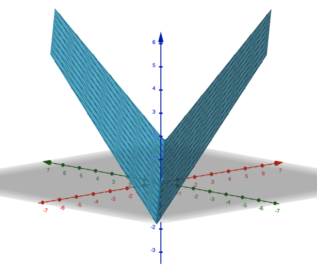
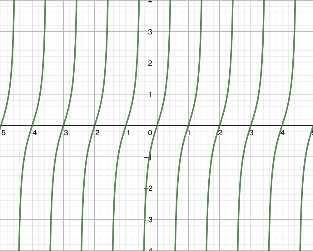
Taking the absolute value simply turns the plane into a v shape with the width of the v shape determined by k. If k=0, then it is simply a vertical plane. Here is the plot of the above function.

A Tiny Bit of Trigonometry

We define k as:

As a trigonometry reminder, the tangent function looks like this:

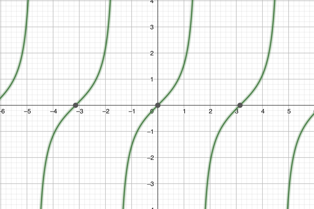
It is bound between (-𝝅/2, 𝝅/2). The limit of tan(x) = -∞ as x approaches -𝝅/2 and ∞ as x approaches 𝝅/2. When we multiply direction by 𝝅 before taking the tangent, we increase the frequency. Now the limit of tan(x) = -∞ as x approaches -0.5 and ∞ as x approaches 0.5

Defining k in this way creates a cyclical function. However, there is a negative side effect. As x approaches 0.5, the output of tan(x*𝝅) becomes very large. We can normalize if we divide everything by k. To avoid a negative k, we square k and then take the square root (this works as long as we are not working with imaginary numbers). To avoid a 0, we simply add 1.

Putting the Math Together

This gets us back to:

In this equation, if k=0 (tan(𝝅) = 0), then the equation simplifies to:

k could also be a very large number (tan(𝝅/2*0.99999999999999)). In this case, as k goes toward infinity, then the equation simplifies to this.

The final step in the line function is:

return 1 - step(width*0.5, distance);

This uses the step function, which converts a floating point number into 0 or 1 based on the threshold. The function takes two parameters, a threshold and a value. If the value is less than the threshold, the output is 0. But if the threshold is greater than or equal to the threshold, then the function returns 1. We invert the output by taking 1 – step.

The Main Function of the OSL Shader: The Search Begins

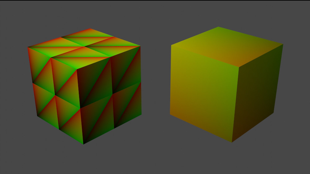
Before we dive into the code, I wanted to give a very important note that is specific to Blender. First, make sure that you unwrap your mesh before you start trying to render. Second, I added one additional input to the function, which is a vector called inputUV. I included this because, by default, Blender seems to use UV by face. Here is an example.

shader basic_shader(
    vector inputUV = vector(0.0,0.0,0.0),
    output color basic_uv = color(0.0, 0.0, 0.0),
    output color out_color = color(0.0, 0.0, 0.0)
    )
{
    // Use the OSL global variables U, V
    basic_uv = color(u,v,0);
    
    // Use the input vector
    out_color = color(inputUV[0],inputUV[1],0);
}

On the left, we use the UV global variables in OSL. The right uses an input vector connected to the UV input node.

Pseudocode

Let’s start with a high level walkthrough of what the script is doing. Below is pseudocode simplifying the steps:

Create a search grid
Determine the number of cells around the current cell to search
Get the current cell of the point we are shading
Assume this is not a scratch point (set scratch to false)

Begin the search:
    For x cells
        For y cells
            Get a “random” point within the search cell
            Get a “random” direction

            Check if there is a line between the “random” point and the current point 
                If yes, add roughness anisotropy to the output. If no, keep looking.

I put “random” in quotes. As discussed above, we are using the hashnoise function (see section above). Now onto the actual code.

The Settings

The code starts by creating our search settings.

It sets a macro to set the number of divisions at 40. This could potentially be exposed as a parameter to the user.

#define DIVISION 40

The variable delta is set to 1/(DIVISION-1), which, in this case, creates a grid of 40 cells each of size delta (with 40 cells, delta = 0.0256).

Next, we determine how many cells we are going to search. We create a radius by taking the square root of the density. Then we get the search cells by dividing by the cell size (delta). To make this an integer, we take the ceiling (basically round up to the next integer). This results in a search size of 13.

We find our current cell (index) by dividing u and v by delta and rounding. Remember that u and v are floating point numbers between [0, 1]. Therefore, if u=0, then u/delta = 0. If u=1, then u/delta = 39.

The Search

Now, we begin the search. We set the variable “scratch” to 0 (basically false). This is the variable that we will use to determine whether there is a scratch at the current point or not. We set roughness and anisotropy to default values.

The search will loop through all cells that are +/- max_search_cell around the current cell. We have a nested loop:

for (int x = -max_search_cell; x <= max_search_cell; ++x){
    for (int y = -max_search_cell; y <= max_search_cell; ++y){
    }
}

Next, we start each loop iteration by setting the current_index (i.e., the cell we are looking at):

current_index = index + point(x, y, 0);

We create a “random” origin point within the search cell. Multiplying by delta converts the cell index back into an actual position on the UV map.

current_origin_p = (current_index + (hashnoise(current_index) - 0.5)) * delta;

Next, we create a “random” direction. I am not sure in this case why the author of this code added a vector(123, 456, 0). This could potentially be exposed to the user as an input to allow further customization of the look.

direction = hashnoise(current_index + vector(123, 456, 0));

Calling the Line Function

Now we call the line function that we discussed above. As the input, we subtract shading_p from current_origin_p. This creates a vector in the direction between our current shading point and the “random” origin point we created in the search cell. We are essentially asking, “Is this point part of a line?”

scratch = line(
    current_origin_p - shading_p,
    current_origin_p - shading_p,
    direction,
    width * hashnoise(current_index));

Tis But a Scratch

The scratch function returns 0 or 1. 0 if our current point is outside of the width threshold and 1 if it is within the width threshold. If 0, we go onto the next cell. Otherwise, if 1, we set the roughness to a value somewhere between min and max and the anisotropy to a value between min and max, and we stop searching. 

if (scratch)
{
    roughness = roughness_default + mix(
        roughness_min,
        roughness_max,
        hashnoise(current_index + vector(123, 456, 1)));

    anisotropic = anisotropic_default + mix(
        anisotropic_min,
        anisotropic_max,
        hashnoise(current_index + vector(123, 456, 2)));
    
    break;
}

The final step is to set the output. This script packs all output into one color variable.

• Red = roughness
• Green = direction of anisotropy
• Blue = anisotropy

Personally, I would prefer three floating point outputs. When I use this, I always have to look at the code or at the github readme to remember which colors are aligned to which outputs.

Anisotropy

What is anisotropy? This was surprisingly harder to answer than I thought. There are many examples, such as brushed metal or wood grains. Below is an example from the Blender Manual.

However, the actual definitions tend to be very detailed. For example “anisotropy is caused by a micro structure, in which long, thin features are aligned in one predominant direction.”

The best definition I could find was the comparison between isotropic: “Properties of a material are identical in all directions” and anisotropic: “Properties of a material depend on the direction; for example, wood. In a piece of wood, you can see lines going in one direction; this direction is referred to as “with the grain”.

Test Renders of the OSL Shader

With our code complete, we can start rendering. Below are some test renders with different densities (0.01 and 0.001).

Hopefully, you found this overview helpful. Please let me know in the comments. Also feel free to send me any other OSL scripts that you would like me to do a deep dive on.

Thank you!